Calculate lethal dosage, resistance ratios, and regression coefficients and tests for linearity
Source:R/ratios.R
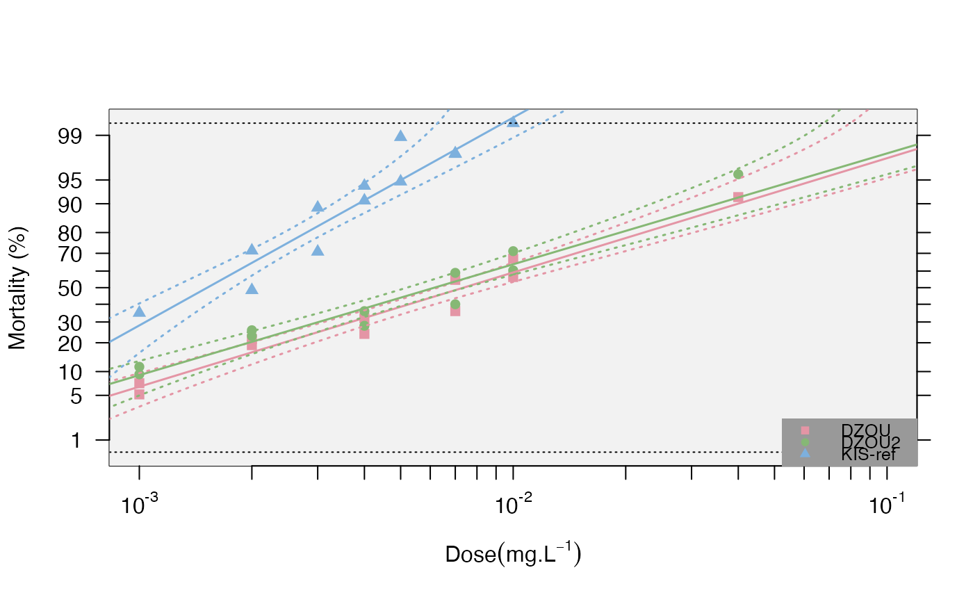
resist.ratio.RdUsing a generalized linear model (GLM, logit link function), this function computes the lethal doses for 25 of the population (LD25, LD50 and LD95, resp.), and their confidence intervals (LDmax and LDmin, 0.95 by default). See details for more info.
Arguments
- data
a data frame of probit-transformed mortality data using the function probit.trans()
- conf.level
numerical. level for confidence intervals to be applied to the models (default 0.95)
- LD.value
numerical. Level of lethal dose to be tested. default=c(25,50,95)
- ref.strain
character. name of the reference strain if present (see details)
- plot
logical. Whether to draw the plot. Default FALSE
- plot.conf
logical. If plot=TRUE, whether to plot the 95 percent confidence intervals. Default TRUE
- test.validity
logical. If plot=TRUE (default), the regression for a strain that failed the linearity test is not plotted
- legend.par
arguments to be passed on to
legend()as inmort.plot()- ...
parameters to be passed on to graphics for the plot (e.g. col, pch)
Value
Returns a data frame with the various estimates mentioned above. If plot=TRUE, plots the mortality on a probit-transformed scale against the log_10 doses.
Details
If a name is provided in ref.strain=, it will be used as the reference to compute the resistance ratios (RR). Alternatively, the function will look for a strain with the suffix "-ref" in the dataset. If this returns NULL, the strain with the lowest LD50 will be considered as reference.
In addition to LD values, the function in a nutshell uses a script modified from Johnson et al (2013), which allows taking the g factor into account ("With almost all good sets of data, g will be substantially smaller than 1.0 and seldom greater than 0.4." Finney, 1971) and the heterogeneity (h) of the data (Finney, 1971) to calculate the confidence intervals (i.e. a larger heterogeneity will increase the confidence intervals). It also computes the corresponding resistance ratios (RR), i.e. the ratios between a given strain and the strain with the lower LD50 and LD95, respectively for RR50 and RR95 (usually, it is the susceptible reference strain), with their 95 Robertson and Preisler (1992). Finally, it also computes the coefficients (slope and intercept, with their standard error) of the linear regressions) and tests for the linearity of the dose-mortality response using a chi-square test (Chi(p)) between the observed dead numbers (data) and the dead numbers predicted by the regression (the test is significant if the data is not linear, e.g. mixed populations).
References
Finney DJ (1971). Probitanalysis. Cambridge:Cambridge University Press. 350p.
Hommel G (1988). A stage wise rejective multiple test procedure based on a modified Bonferroni test. Biometrika 75, 383-6.
Johnson RM, Dahlgren L, Siegfried BD, Ellis MD (2013). Acaricide,fungicide and drug interactions in honeybees (Apis mellifera). PLoSONE8(1): e54092.
Robertson, J. L., and H.K. Preisler.1992. Pesticide bioassays with arthropods. CRC, Boca Raton, FL.
Examples
data(bioassay)
transd<-probit.trans(bioassay$assay2)
data<-transd$tr.data
resist.ratio(data,plot=TRUE)

#>         Slope SlopeSE Intercept InterceptSE    h      g Chi2 df Chi(p)   LD25
#> DZOU     1.75  0.1537      3.72      0.3579 1.91 0.0397 9.88 10 0.4514 0.0030
#> DZOU2    1.69  0.1657      3.74      0.3907 2.33 0.0490 9.92 10 0.4473 0.0025
#> KIS-ref  3.17  0.3812      8.95      0.9849 3.26 0.0716 8.59 11 0.6597 0.0009
#>         LD25min LD25max   LD50 LD50min LD50max   LD95 LD95min LD95max rr25
#> DZOU      2e-04  0.0192 0.0074   6e-04  0.0404 0.0645  0.0087  0.2472 3.24
#> DZOU2     1e-04  0.0194 0.0062   3e-04  0.0412 0.0576  0.0055  0.2578 2.64
#> KIS-ref   0e+00  0.0142 0.0015   0e+00  0.0209 0.0050  0.0001  0.0537 1.00
#>         rr25min rr25max rr50 rr50min rr50max rr95 rr95min rr95max
#> DZOU     2.7000    3.91 4.84  4.1600    5.64   13  7.6800   22.00
#> DZOU2    2.1900    3.18 4.05  3.5000    4.69   11  7.1100   19.00
#> KIS-ref  0.7947    1.26 1.00  0.8488    1.18    1  0.8085    1.24